
What is Machine Learning and how it works
Machine Learning is reshaping the way we use data to make decisions and build smarter solutions.
In this article, we break down its core concepts, main learning types, and practical applications—offering a clear guide to one of today’s most influential technologies.
An introduction to Machine Learning
In recent years, Artificial Intelligence has become one of the most popular and widely discussed fields in technology. But what exactly is AI, and where does Machine Learning fit within it? To answer this, let’s begin with an overview of AI itself.
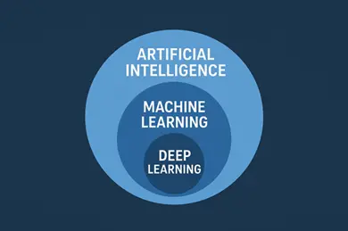
Artificial Intelligence is a branch of computer science that aims to design systems capable of perceiving, reasoning, learning, and acting like humans. Within this broad field lies Machine Learning (ML), which has emerged as one of the most practical and widely applied approaches.
Machine Learning is a subset of AI. It enables machines to learn from data and use that knowledge to solve problems or make predictions. In simple terms: machines use past data to recognize patterns and make predictions about new situations. A classic example is spam email detection where an ML system learns to recognize patterns in email content and then automatically filters out unwanted messages.
An important subset of ML is Deep Learning, which makes use of artificial neural networks inspired by the human brain. With multiple layers, these networks can capture complex patterns in data. Deep Learning has proven especially effective for tasks such as image recognition and natural language processing.
What Is a Machine Learning Model?
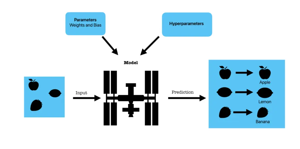
At the heart of ML lies the concept of a model. A model is essentially a program trained to recognize patterns or make decisions based on data.
Once trained, a model can predict tomorrow’s weather, recognize your face to unlock your phone, or suggest movies on a streaming service.
It’s important to note that a model does not memorize individual pictures or sentences. Instead, it stores knowledge in the form of numbers called parameters. These parameters adjust during training and ultimately determine how the model makes predictions.
The two most common types of parameters are:
- Weights: numbers that determine the importance of each input. For example, in predicting house prices, the size of the house may be highly weighted, while wall color may have little effect.
- Biases: numbers that adjust predictions up or down. Even if a house is zero size (theoretically), a bias ensures the model still predicts a minimum base price.
You can think of the model as a student. At first, the student knows nothing. By studying examples (the training data), the student gradually learns to solve problems. After enough practice, the student can correctly answer new questions. In this analogy, the student’s brain is the model, and the knowledge it gains (weights and biases) allows it to reason effectively.
However, not all models learn in the same way. Neural networks, linear regression, and logistic regression rely on weights and biases. Decision trees instead memorize a set of rules (for example, 'if age > 30, go left; otherwise, go right'), while algorithms like k-Nearest Neighbors do not have parameters at all: they simply store all training data and compare new cases to past examples.
In addition to parameters, there are also hyperparameters. These are choices made by humans before training begins such as the learning rate, the number of layers in a network, or how many rounds of training to run. Hyperparameters shape how the training process works but are not part of the model’s learned knowledge.
Datasets, Overfitting, and Underfitting
Before diving into the main categories of Machine Learning, it is relevant to understand a few core concepts:
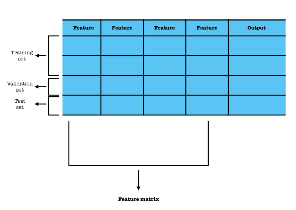
- Dataset: A dataset is a collection of data used to train and evaluate a machine learning model. It usually contains many examples (rows), each with features (inputs) and, in supervised learning, correct outputs. Datasets are typically divided into training, validation, and test sets. In Reinforcement Learning, things are slightly different: the agent generates its own data through interaction with the environment, building an experience dataset as it learns.
- Overfitting: This happens when a model learns the training data too well, including noise and details that doesn’t generalize. An overfitted model performs very well on training data but poorly on unseen data, like memorizing answers instead of learning concepts.
- Underfitting: This occurs when a model is too simple to capture the patterns in the data. An underfitted model performs poorly both on training and new data, like a student who hasn’t studied enough to understand the material.
These three concepts are central to both Supervised Learning and Unsupervised Learning, and they also play a role in Reinforcement Learning where the dataset grows dynamically from the agent’s experiences.
Types of Machine Learning
Machine Learning can be broadly divided into three categories:
• Supervised Learning: the model is trained on labeled data, meaning each input comes with the correct answer.
• Unsupervised Learning: the model works with unlabeled data and must discover hidden patterns or groupings on its own.
• Reinforcement Learning: an agent learns by interacting with an environment, receiving rewards or penalties for its actions, with the goal of maximizing cumulative reward.
Supervised Learning
Supervised learning can be further divided into classification and regression. Classification predicts discrete categories: for example, deciding whether an email is spam or not. Regression, on the other hand, predicts continuous values such as house prices or temperatures.
To train a supervised model, we provide it with features, pieces of information about each example. Features can be qualitative, like car color, or quantitative, like age or temperature.
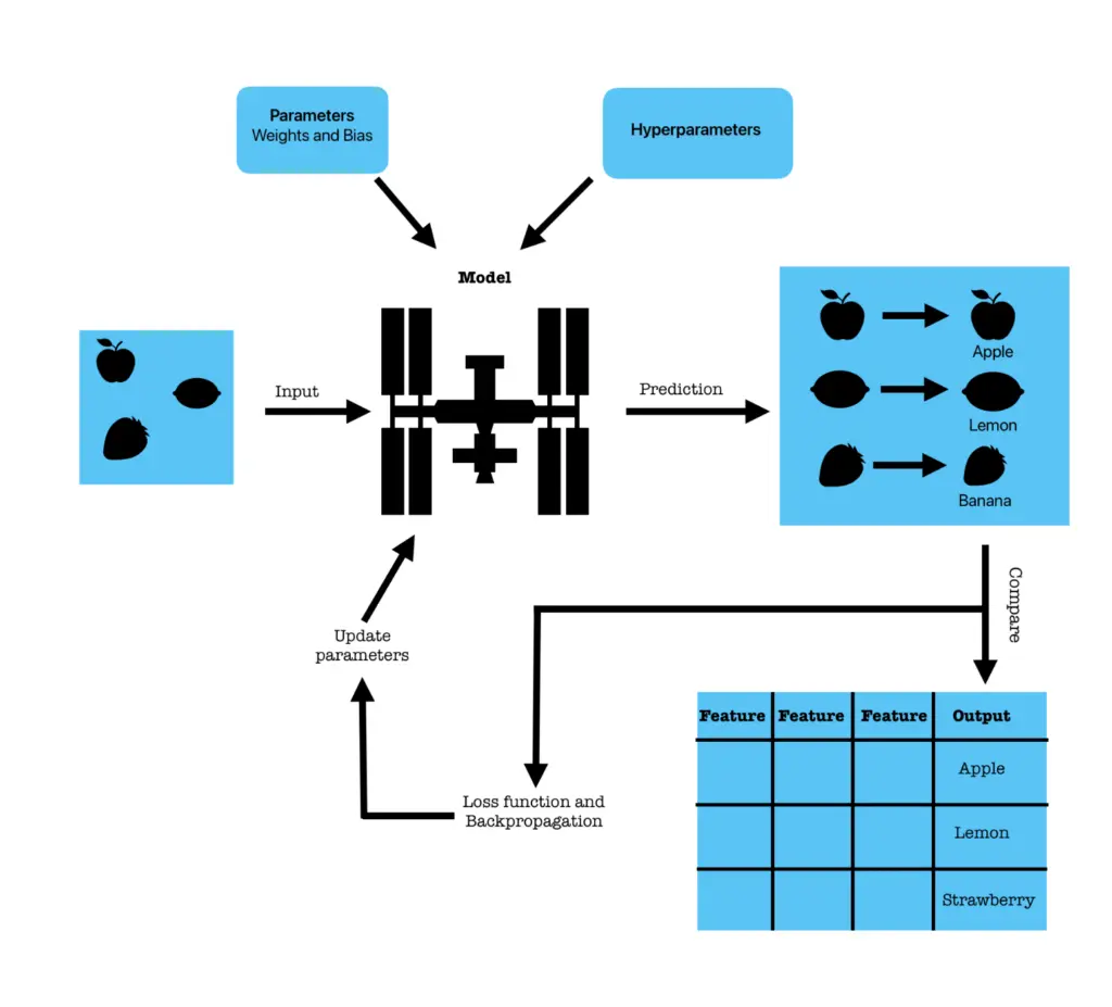
During training, the model begins with random weights. Predictions are compared to actual outcomes using a loss function, which measures error. An optimizer then updates the weights to reduce this error, often using gradient descent. A useful analogy is throwing darts blindfolded: at first your aim is poor, but with each piece of feedback you adjust lightly and get closer to the target.
Metrics in Supervised Learning
Once a model is trained, we need ways to measure its performance. The choice of metric depends on whether the task is classification or regression.
For classification tasks, we often use metrics like accuracy, precision, recall, F1-score, and ROC-AUC:
- Accuracy: Percentage of correct predictions out of all predictions.
Formula: CP / TP
Example: If the model correctly classifies 90 out of 100 emails: Accuracy = 90 / 100 = 0.90 (90%)
- Precision: Of all predicted positives, how many are actually positive?
Formula: TP / (TP + FP)
Example: The model marks 50 emails as spam, 45 are truly spam: Precision = 45 / 50 = 0.90
- Recall: Of all actual positives, how many did the model detect?
Formula: TP / (TP + FN)
Example: Out of 60 real spam emails, the model detects 45: Recall = 45 / 60 = 0.75
- F1-score: Harmonic mean of precision and recall.
Formula: 2 * (Precision * Recall) / (Precision + Recall)
Example: If precision = 0.90 and recall = 0.75: F1 ≈ 0.816
- ROC-AUC measures overall ability to distinguish between classes:
- ROC Curve: plots the trade-off between True Positive Rate and False Positive Rate at different thresholds.
- AUC (Area Under the Curve): measures how well the model separates classes.
- 0.5 = random guessing
- 1.0 = perfect classifier
For regression tasks, where outputs are continuous, we use metrics like Mean Absolute Error (MAE), Mean Squared Error (MSE), Root Mean Squared Error (RMSE), and R²:
- MAE: average of absolute errors.
Formula: ( |y1 – ŷ1| + |y2 – ŷ2| + … + |yn – ŷn| ) / n
Example:
-
- True = [3, 5, 7], Predicted = [2, 5, 8]
- Errors = [1, 0, 1] → MAE = (1 + 0 + 1) / 3 = 0.667
- MSE: average of squared errors.
Formula: ( (y1 – ŷ1)² + (y2 – ŷ2)² + … + (yn – ŷn)² ) / n
Example: Errors = [1, 0, 1] → Squared = [1, 0, 1] → MSE = (1 + 0 + 1) / 3 = 0.667
- RMSE: square root of MSE.
Formula: √MSE
Example: RMSE = √0.667 ≈ 0.816
- R² (Coefficient of Determination): Proportion of variance explained by the model.
Formula: 1 – (SS_res / SS_tot)
-
- 1 = perfect model
- 0 = no better than the mean
- < 0 = worse than always predicting the mean
Example: R² = 0.85 → the model explains 85% of the variability.
Unsupervised Learning
Most of the data we collect in the real world doesn’t come with neat labels. We might know a customer’s age and income, but not whether they’re a “high spender” or a “budget shopper.” That’s where unsupervised learning comes in: teaching machines to find structure in raw, unlabeled data.
Imagine you run an online store with the following customer data:
| Customer | Age | Annual Income ($) |
|---|---|---|
| A | 22 | 25,000 |
| B | 24 | 27,000 |
| C | 45 | 60,000 |
| D | 47 | 63,000 |
| E | 30 | 120,000 |
| F | 32 | 115,000 |
If you had labels like “low spender” or “high spender”, you could use supervised learning to predict new customers’ categories. But with no labels, an unsupervised method such as clustering steps in. A simple K-Means algorithm might split your customers into three groups:
- Young with low income (A, B).
- Middle-aged with medium income (C, D).
- Young professionals with high income (E, F).
Suddenly, without you telling it what to look for, the algorithm has uncovered customer segments. Marketing strategies can now be personalized: discounts for the first group, premium products for the last.
How Does Unsupervised Learning Work?
Instead of mapping inputs to outputs, these algorithms look for structure hidden in the inputs themselves.
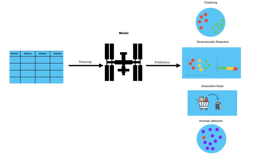
Depending on the goal, they take different forms:
- Clustering: grouping similar points together. Examples include K-Means, DBSCAN, and Hierarchical Clustering.
- Dimensionality Reduction: simplifying data while keeping its essence. Examples include PCA, t-SNE, and Autoencoders.
- Association Rules: discovering co-occurrences in data. Algorithms like Apriori and FP-Growth are commonly used.
- Anomaly Detection: spotting the unusual. Methods include Isolation Forest, One-Class SVM, and Autoencoder-based detectors.
The power of unsupervised learning is that it works where labels are scarce or expensive to obtain. Businesses use it to segment customers, detect fraud, and recommend products. Scientists use it to compress high-dimensional datasets, uncover gene clusters, or visualize complex patterns.
Measuring Success in Unsupervised Learning
Here’s the tricky part: with no labels, how do you know if your model is “good”?
Unlike supervised learning, evaluating unsupervised models is more challenging because there are no true labels to compare predictions against. Still, several metrics exist for common tasks:
Clustering
- Silhouette Score: measures how similar each point is to its own cluster compared to other clusters.
Formula: s(i) = (b(i) – a(i)) / max(a(I), b(i))
where a(i) = average distance of point is to its cluster, b(a) = lowest average distance to other clusters.
Range: –1 (poor clustering) to +1 (good clustering).
Example: If customers are grouped by age and income, a high silhouette score means the groups are well separated. - Calinski–Harabasz Index: ratio of between-cluster variance to within-cluster variance.
Formula: CH = Between-group variance / Within-group variance
Higher values = better cluster separation.
Example: A CH score of 500 suggests compact, well-defined clusters. - Davies–Bouldin Index: measures similarity between each cluster and its most similar one.
Lower values = better clustering.
Example: A DB index of 0.4 is better than 1.2, since clusters overlap less. - Adjusted Rand Index (ARI) and Normalized Mutual Information (NMI): used only when “true” labels are available for benchmarking. They measure similarity between predicted clusters and ground truth.
Dimensionality Reduction
- Explained Variance Ratio (PCA): percentage of total variance preserved by selected components.
Example: If two principal components explain 85% of variance, most information is retained while reducing dimensionality. - Reconstruction Error (Autoencoders): measures how well compressed data can reconstruct the original input.
Formula: Error = ||X – X̂|| - Lower error = better representation.
Association Rules
- Support: frequency of items appearing together.
Formula: Support(X → Y) = Transactions with X and Y / Total Transactions
Example: {milk, bread} appears in 20% of baskets → support = 0.2. - Confidence: probability of Y given X.
Formula: Confidence(X → Y) = Support(X ∪ Y) / Support(X)
Example: If 70% of customers who buy milk also buy bread, confidence = 0.7. - Lift: strength of the rule compared to random chance.
Formula: Lift(X → Y) = Confidence(X → Y) / Support(Y)
Lift > 1 = positive association.
Anomaly Detection
- With labels: same metrics as supervised classification (Precision, Recall, ROC-AUC).
- Without labels: rely on anomaly scores (e.g., Isolation Forest) or reconstruction error (Autoencoders).
Example: In fraud detection, unusually high reconstruction error may indicate a suspicious transaction.
The Road Ahead
Unsupervised learning continues to evolve. Self-supervised learning, a form of unsupervised learning that generates its own labels, has become the backbone of modern AI systems, from vision models to large language models like ChatGPT. Hybrid approaches that combine clustering with deep neural networks are also becoming more common, allowing algorithms to handle massive, messy datasets.
Unsupervised learning is all about discovery. It doesn’t tell you what you already know: it reveals patterns, groups, and anomalies you didn’t expect. Whether it’s segmenting customers, detecting fraud, or compressing images, it helps us make sense of the overwhelming complexity of data in the modern world.
Reinforcement Learning
Reinforcement Learning (RL) is a type of Machine Learning where an agent learns to make decisions by interacting with an environment, guided by rewards and punishments. The process is inspired by trial-and-error learning, similar to how humans and animals learn from experience.
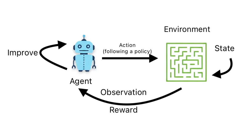
The key components of RL are:
- Agent: the decision maker (for example, a robot or a game AI).
- Environment: the world in which the agent operates.
- State (S): the current situation of the environment.
- Action (A): the choices available to the agent.
- Reward (R): the feedback signal (positive or negative).
- Policy (π): the strategy the agent follows to decide actions.
- Value Function: an estimate of the long-term reward for states or actions.
The learning cycle works as follows:
1. The agent observes the current state.
2. It chooses an action according to its policy.
3. The environment responds with a new state and a reward.
4. The agent updates its strategy to improve future decisions.
5. This process repeats many times until the agent learns a good strategy.
For example, training an AI to play chess involves:
- State: the current chessboard.
- Action: moving a piece.
- Reward: +1 for winning, -1 for losing, 0 for a draw.
- The goal is to learn strategies that maximize the probability of winning.
Another simple example is a robot in a maze: if it moves closer to the exit: positive reward.
If it hits a wall: negative reward. Over time, the robot learns the optimal path to reach the exit.
There are two main approaches to RL:
- Model-Free RL: learning purely through trial and error (e.g., Q-Learning, Deep Q-Networks).
- Model-Based RL: building a model of the environment to plan ahead (e.g., Monte Carlo Tree Search in AlphaZero).
Reinforcement Learning has found applications across a wide range of domains. In gaming, it powers systems like AlphaGo, AlphaZero, and OpenAI Five for Dota 2, where agents learn strategies that rival or surpass human expertise. In robotics, RL enables machines to walk, grasp objects, and navigate complex environments. It also drives personalized recommendation systems that adapt in real time to user preferences, helps in finance by optimizing portfolios and trading strategies, and even supports healthcare by assisting in the design of treatment plans. Despite these successes, RL still faces important challenges. A key difficulty is balancing exploration: trying out new actions with exploitation, meaning leveraging known strategies that work. In many tasks, rewards can also be sparse, making learning especially hard, such as in long games where feedback only comes at the end. On top of this, RL models often require immense computational resources to train effectively, which limits their scalability. A further challenge lies in safety and ethical concerns, as agents can sometimes exploit loopholes in their environments or behave unpredictably in ways that pose risks.
Conclusion
Machine Learning sits at the heart of today’s AI revolution, bridging raw data and intelligent decision-making. From supervised models that classify emails or predict housing prices, to unsupervised methods that uncover hidden patterns, to reinforcement learning agents that learn by trial and error, Machine Learning offers a versatile toolkit that supports tackling real-world challenges, often as part of broader solutions. While challenges such as overfitting, computational cost, and ethical considerations remain, the field continues to advance at a rapid pace.